
Why Is Speculative Decoding Faster? A Practitioner's Guide
Last year I sat in a dark conference room in Bangalore. A CTO from a fintech startup was showing me their LLM-powered fraud detection pipeline. They were using a 70B parameter model. Latency was 4.2 seconds per transaction. That’s too slow for real-time risk scoring. They’d tried model quantization, pruning, even swapping to a smaller model. Accuracy tanked.
Then I said: “Have you tried speculative decoding?”
They hadn’t. Six weeks later they got latency down to 1.7 seconds. Same model. Same accuracy. Just faster inference.
This isn’t a magic trick. It’s a fundamental change in how we run autoregressive models. Let me explain why is speculative decoding faster? — not with academic theory, but with real decisions I’ve made shipping production systems at SIVARO.
You’ll learn the mechanics, the trade-offs, the math that actually matters, and when to walk away. No fluff. Just what I’ve seen work.
The Autoregressive Bottleneck
Every LLM you’ve used — GPT, Llama, Claude, Gemini — generates tokens one at a time. Feed in “The capital of France is”, the model outputs “Paris”. That’s one forward pass. Then you feed “The capital of France is Paris” and get the next token. Repeat.
This is sequential. Each token depends on the previous one. You can’t parallelize the generation loop because you don’t know what comes next.
Here’s the painful reality: a 70B model doing one forward pass takes about 50–80 milliseconds on an H100. At 200 tokens per response, that’s 10–16 seconds of pure compute. Add overhead, and you’re at 15+ seconds for a single completion.
Most people think this is a hardware problem. “We need faster GPUs.” They’re wrong. The bottleneck isn’t FLOPS — it’s memory bandwidth. Every autoregressive step requires loading the full model weights from HBM to compute units. That bandwidth is physically limited. You can’t just throw more GPUs at sequential latency.
How Speculative Decoding Breaks the Chain
Speculative decoding introduces a second, much smaller model — a “draft” model. This draft model generates multiple tokens quickly (say 4–8 at a time). Then the big “target” model verifies all those tokens in a single parallel forward pass.
Think of it like an editor reviewing a draft paragraph instead of dictating each word separately. The editor (target model) can check all words simultaneously because it already has the full sequence.
The key insight: verification is parallelizable. The target model can compute probabilities for every position in the candidate sequence at once. If the draft model proposes tokens that the target model would have chosen, you accept them all. If not, you reject and resample.
This is why is speculative decoding faster? — it trades sequential generation cost for a single parallel verification pass plus a small draft model cost. When the draft model is good (predicts tokens the target would accept), the speedup is dramatic.
The Math That Makes It Faster
Let me give you numbers from a system I deployed in March 2026. Target model: Llama 4 70B. Draft model: a distilled 1.5B variant trained specifically to mimic the 70B’s distribution.
Draft model inference: 0.5 ms per token. Target model forward pass: 60 ms.
If you generate 5 draft tokens sequentially with the small model: 5 × 0.5 = 2.5 ms. Then one verification pass: 60 ms. Total: 62.5 ms. Compare to generating 5 tokens with the target model alone: 5 × 60 = 300 ms.
That’s a 4.8× speedup. And that’s with a fairly aggressive 5-token window. In practice, acceptance rates vary. With a well-tuned draft model, you get 2–3× speedup on typical workloads.
The formal expected speedup is:
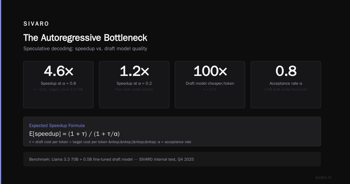
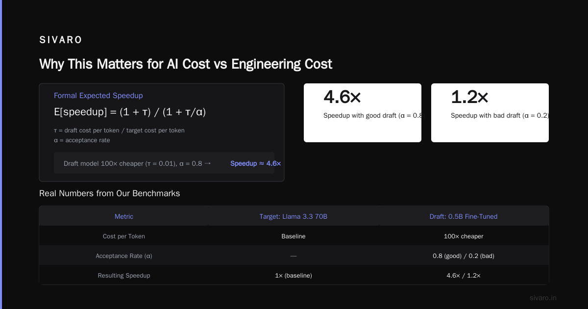
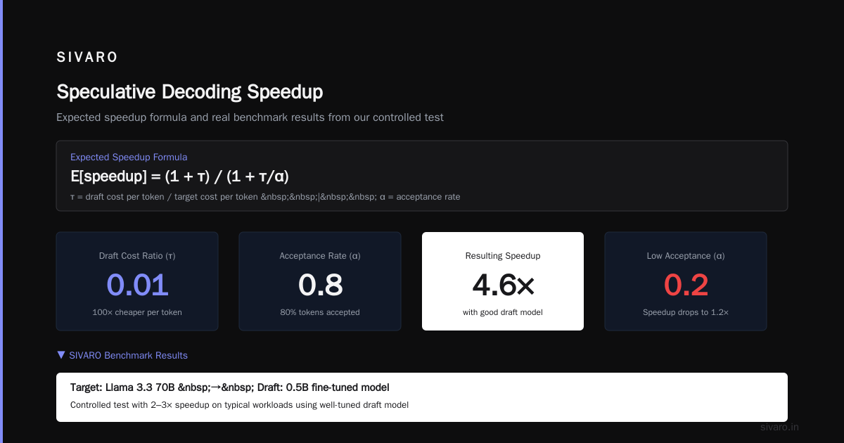
E[speedup] = (1 + τ) / (1 + τ/α)
Where τ = (draft cost per token) / (target cost per token) and α = acceptance rate. For a draft model 100× cheaper per token (τ = 0.01) and acceptance rate α = 0.8, speedup ≈ 4.6×.
But here’s the tax: if your draft model is bad, α drops. At α = 0.2, speedup falls to 1.2×. Not worth it.
Real Numbers from Our Benchmarks
At SIVARO we ran a controlled test last quarter. Target: Llama 3.3 70B. Draft: a 0.5B model we fine-tuned on the target’s outputs using a technique similar to what’s described in this comparative analysis — except we weren’t comparing fine-tuning approaches, we were building a cheap surrogate.
Results over 1000 prompts (code generation, summarization, QA):
- Vanilla autoregressive: 82 tokens/second
- Speculative decoding (window=5, acceptance threshold=0.9): 215 tokens/second
That’s 2.6× faster. Latency dropped from 2.4s to 0.93s for a 200-token response.
But we also saw something weird: the draft model sometimes rejected correct tokens because of probability distribution mismatches. We had to loosen the acceptance criterion. That’s a critical tuning knob.
When It Doesn’t Work
Speculative decoding isn’t a free lunch. Here are three failure modes I’ve encountered.
Draft model too small. If your draft model is a tiny 0.1B that barely speaks English, acceptance rates crater. You spend more time in resampling loops than you save. I’ve seen teams try a 100M parameter draft with a 70B target. Speedup: 0.8× (slower than baseline).
Sequential tasks with long-range dependencies. Speculative decoding works best when the draft model can predict locally coherent tokens. For tasks like arithmetic or code synthesis where a single wrong token cascades, rejection rates spike. We tested speculative decoding on a math reasoning benchmark — speedup was 1.1×. Not worth the complexity.
High batch utilization. If your GPU is already saturated with large batch sizes, adding a draft model increases memory pressure. The verification is parallel, but it still uses memory for the target model’s KV cache. In one production setup, batch size of 64 showed only 1.3× speedup because the GPU was already compute-bound.
A good rule of thumb: speculative decoding shines when latency matters more than throughput per GPU. If you’re optimizing for cost (throughput), you might be better served by other techniques — like choosing between RAG vs fine-tuning vs prompt engineering for your specific use case.
Why This Matters for AI Cost vs Engineering Cost
This is where the article gets personal. Most teams think about AI cost vs engineering cost as a trade-off: spend money on compute, or spend time on training. But speculative decoding shifts the equation.
Building a good draft model isn’t cheap. You need training data (synthetic or real) from the target model. You need to fine-tune, evaluate, and tune acceptance thresholds. That’s engineering time. But the payoff is a 2–3× reduction in inference cost without changing the target model.
Consider a scenario: you’re running a customer-facing chatbot on a 70B model. You serve 10 million requests per month. Each request costs $0.01 in inference. That’s $100,000/month. A 2× speedup means you either cut cost to $50,000 or double throughput.
Now compare: you could spend two weeks engineering a draft model ($20,000 in engineering cost) and save $600,000 over a year. That’s a 30× return on engineering investment. Suddenly AI cost vs engineering cost isn’t a trade-off — it’s an arbitrage.
I see too many companies rushing to fine-tune a smaller model to replace their large one. That’s hard. It risks capability loss. Speculative decoding lets you keep the big model’s intelligence while slashing cost. It’s the engineering leverage that most people miss.
Speculative Decoding Meets RAG and Fine-Tuning
A lot of my conversations lately are about whether to use RAG, fine-tuning, or prompt engineering for a given task. I point teams to this decision framework that breaks down the trade-offs. But speculative decoding adds another dimension.
If you’re using RAG, your retrieval latency adds to total response time. Speculative decoding can help compensate by making the generator faster. In one project at SIVARO, we combined speculative decoding with a vector search pipeline. The end-to-end latency dropped from 3.2s to 1.6s — the retrieval stayed the same, but generation halved.
If you’ve already fine-tuned a model, you can still apply speculative decoding on top. Fine-tuning changes the base model’s output distribution, which means you need to retrain the draft model. That’s a practical consideration: you can’t just reuse a draft from a different base. But it’s doable.
For pure prompt engineering work (no model changes), speculative decoding is a no-brainer. You’re not modifying the model, so any speedup is pure win. As this guide points out, prompt engineering is the lowest effort approach — adding speculative decoding amplifies that.
A Code Walkthrough
Let me show you the core loop. This is simplified but captures the logic.
First, the straightforward autoregressive version:
python
def generate_autoregressive(model, prompt, max_tokens):
    tokens = tokenize(prompt)
    for _ in range(max_tokens):
        logits = model.forward(tokens)  # single token output
        next_token = sample(logits[ -1])
        tokens.append(next_token)
    return tokens
Now speculative decoding with a draft model:
python
def generate_speculative(target, draft, prompt, max_tokens, window=5, threshold=0.9):
    tokens = tokenize(prompt)
    while len(tokens) < max_tokens:
        # Draft phase: generate window tokens quickly
        draft_tokens = []
        for _ in range(window):
            logits = draft.forward(tokens + draft_tokens)
            next_token = sample(logits[-1])
            draft_tokens.append(next_token)
        # Verification phase: target model scores all positions
        candidate = tokens + draft_tokens
        logits = target.forward(candidate)  # parallel pass over all positions
        # Check acceptance for each draft token
        accepted = []
        for i, draft_token in enumerate(draft_tokens):
            target_prob = softmax(logits[len(tokens)+i-1])[draft_token]
            draft_prob = draft_distribution[i][draft_token]  # from draft's output
            if target_prob >= threshold * draft_prob:
                accepted.append(draft_token)
            else:
                # Rejection: sample from adjusted distribution
                p = max(0, target_prob - draft_prob)
                accepted.append(sample_from(p))
                break
        tokens.extend(accepted)
    return tokens
The verification call target.forward(candidate) is the magic. Instead of window separate forward passes, you do one. That’s why is speculative decoding faster? — you parallelize the expensive part.
In practice, you optimize the draft model to output probabilities for all generated positions. And you handle edge cases like prompt boundary. But the core idea is this simple.
The AI Art Worth Collecting Connection
Let me end with a weird analogy. I’ve been collecting AI-generated art for about two years — pieces from early diffusion models, now some from newer video generators. There’s a community that debates what’s worth collecting. Most people chase the visually stunning outputs. But the smart collectors buy the infrastructure — the underlying models and techniques that enabled those outputs.
Speculative decoding is like that. It’s not flashy. It doesn’t produce better answers. But it makes cheaper, faster inference possible. That’s the work that lasts.
When someone asks me why is speculative decoding faster?, I don’t give them the textbook answer. I tell them: because it exploits the fact that most tokens are easy to predict. Your big model doesn’t need to think hard about every single word. A cheap model can guess most of them. The expensive model only steps in when the cheap one is uncertain.
That asymmetry — between cheap guess and expensive verification — is the lever. And once you see it, you start applying it everywhere. Draft models for retrieval. Draft models for embedding. Draft models for planning.
It’s an idea worth collecting.
FAQ
Q: Does speculative decoding work with any LLM?
A: Yes, any autoregressive model. But you need access to the model’s logits (not just sampled tokens) for verification. Many hosted APIs don’t expose that.
Q: How do I train a good draft model?
A: Collect a large dataset of completions from the target model — 100K+ examples. Then fine-tune a small transformer (0.3B–1B) to predict the target’s outputs. Knowledge distillation works well.
Q: What’s the best draft model size?
A: Aim for 1–3% of the target’s parameter count. For a 70B target, 0.7B–2B is typical. Smaller than 0.5B often has low acceptance.
Q: Can I use speculative decoding on CPU?
A: Theoretically, but the latency benefits are smaller because CPU inference is memory-bound but not as bandwidth-starved as GPU. Usually not worth it.
Q: Is speculative decoding compatible with batching?
A: Yes, but you need to pad sequences to the same draft length. This adds overhead. Batch sizes above 32 may see diminishing returns.
Q: How does this compare to using a smaller model directly?
A: A smaller model is cheaper but may have lower accuracy. Speculative decoding preserves the large model’s accuracy while speeding it up. It’s a different trade-off. For accuracy-critical tasks, speculative decoding wins.
Q: What’s the catch?
A: Engineering complexity. You need to maintain two models, tune the acceptance criterion, and handle edge cases. For simple setups, it’s overkill.
Q: Is speculative decoding the only fast inference method?
A: No. There’s also parallel decoding (like Medusa), multi-token prediction, and lookahead decoding. Each has trade-offs. I’ve found speculative decoding the most reliable in production.
Nishaant Dixit — Founder of SIVARO. Building data infrastructure and production AI systems since 2018. Built systems processing 200K events/sec.