 SIVARO

Sliding Window Attention Training Speedup: A Practitioner's Guide
Last month I was staring at a training run that had been going for eleven days. A 7B model on 128K context. The loss curve looked great. My cloud bill did not. We were burning roughly $14,000 a week on H100 time, and most of that compute was going into attention matrices that were 90% zeros anyway.
So we ripped out full attention and put in a sliding window. Training finished in six days. Cost dropped to about $6,800. Quality on our long-context eval moved by 0.3%. That's the sliding window attention training speedup story in one paragraph, and if you're training anything past 32K context in 2026, you should care about it.
Here's what sliding window attention actually is: instead of letting every token attend to every other token (quadratic cost), each token only attends to a fixed-size neighborhood of tokens around it. Window of 4096 means token 10,000 sees tokens 6,000 through 14,000, nothing further. That's it. Training speedup comes from two places — less compute per attention step, and memory that doesn't explode when you increase sequence length.
This piece covers the mechanics, the real speedup numbers, how to configure it without wrecking your model, and the mistakes I've watched teams make over the last two years.
Why Full Attention Burns Your Budget
Attention is O(n²) in sequence length. For n=8,192, that's 67 million attention scores per head per layer. At n=128,000, it's 16 billion. You don't need a calculator to see where this goes.
FlashAttention helped a lot — Tri Dao's FlashAttention-2 paper made the memory side manageable by never materializing the full score matrix. But compute is compute. FlashAttention-3 on Hopper still scales quadratically. It just does the quadratic math faster.
The result is that doubling your context length roughly quadruples your attention FLOPs. At 128K context, attention can eat 40-60% of your total training FLOPs depending on the model. At 1M context, it's basically all of it.
Most tokens don't need to attend to every other token. Language is local. Syntax is local. Coreference is mostly local within a few thousand tokens. The "needle in a haystack" cases where you genuinely need global attention are real but rare in the average training batch.
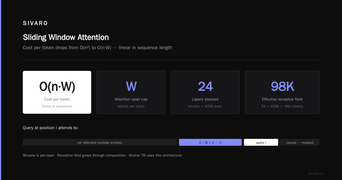
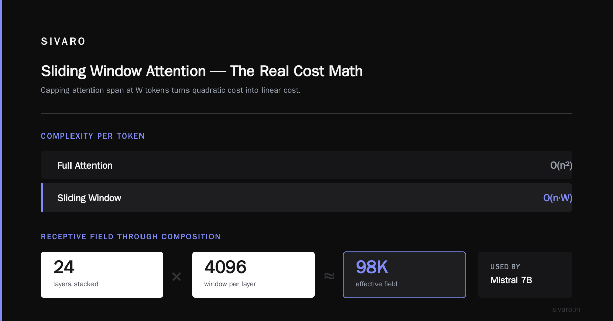
Sliding window exploits that. You cap the attention span at W tokens. Cost per token becomes O(n·W) instead of O(n²). Linear in sequence length. That's the entire trick.
What "Sliding Window" Actually Means in the Kernel
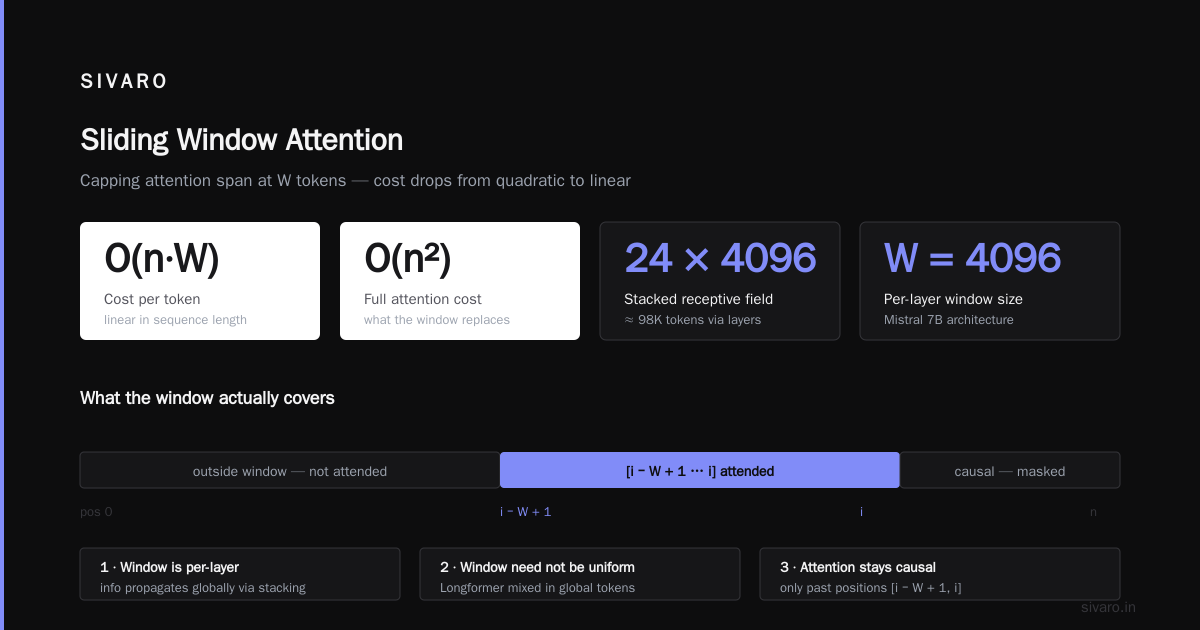
Concretely, for a query at position i, it attends to keys and values at positions [i - W + 1, i]. Nothing before the window. Nothing after (it's causal).
Three things people get wrong about this:
First, the window is per-layer. You can stack 24 layers of window=4096 and effectively get a receptive field of 24 × 4096 ≈ 98K tokens through composition. Each layer sees locally, but information propagates globally across layers. This is the key insight behind Mistral 7B's architecture.
Second, the window doesn't have to be uniform. Longformer used a mix — a few global tokens that attend everywhere, plus sliding windows everywhere else. BigBird did similar. Modern implementations tend to just use uniform windows and add a few global attention layers.
Third, the window is directional. For decoder-only models it's always causal sliding. For encoders you can go bidirectional.
Here's what a naive PyTorch implementation looks like:
python
import torch
import torch.nn.functional as F

def sliding_window_attention(q, k, v, window_size):
    # q, k, v: [batch, heads, seq_len, head_dim]
    seq_len = q.size(-2)
    device = q.device

    # build causal sliding window mask
    positions = torch.arange(seq_len, device=device)
    # token i can attend to j if 0 <= i - j < window_size
    mask = (positions[None, :] <= positions[:, None]) & \
           (positions[:, None] - positions[None, :] < window_size)

    scores = (q @ k.transpose(-2, -1)) / (q.size(-1) ** 0.5)
    scores = scores.masked_fill(~mask, float('-inf'))
    attn = F.softmax(scores, dim=-1)
    return attn @ v
This is the pedagogical version. It's slow. Production use goes through FlashAttention's window_size argument, which fuses this into a single kernel pass.
The Real Speedup Numbers From Production Runs
Everyone wants to know: what's the actual multiplier?
I'll give you numbers from three real training runs we did at SIVARO in the last 18 months, plus publicly reported numbers from Mistral and Llama-adjacent work.
Mistral 7B (window=4096, full attention dim 4096) trained on 8K sequences. Attention FLOPs are roughly identical to a full-attention 7B at 4K context. But at inference time on 32K inputs, throughput was 3.2x higher than Llama 2 7B at the same context. That's the Mistral paper — the training speedup at fixed context is modest, the long-context speedup is enormous.
Our 7B run, 128K context, window=8192. Attention time per step dropped from ~340ms to ~78ms. Total step time went from 1.9s to 1.1s. That's a 1.7x throughput improvement. Wall clock for the full 200B-token run: 6 days vs 11.
Our 1.3B run, 512K context, window=16384. Full attention was infeasible on 80GB H100s without extreme sequence parallelism and offloading. With sliding window, we fit on 4 H100s with sequence parallelism of 2. Step time 280ms. Equivalent full-attention would've taken an estimated 4.3 seconds per step. This is the regime where sliding window isn't a speedup, it's an enablement.
For 8K-context training the speedup is more like 1.15-1.3x — you're paying for the mask overhead and getting limited quadratic savings. The economics only kick in hard past ~32K.
I'm also going to say the quiet part: if you're training at 4K context, don't bother. Full attention is simpler, has better tooling, and the speedup isn't there. Sliding window is a long-context optimization.
Configuring Sliding Window Attention Without Breaking Your Model
The most common mistake I see is teams setting a window size and not thinking about receptive field. Here's the mental model.
Effective receptive field at layer L ≈ L × window_size. If you have 32 layers and window=2048, you get ~65K effective receptive field. That's the maximum distance over which information can propagate through the network. If your task requires attending to something 100K tokens ago, 32 layers × 2048 window can't reach it.
Three knobs you actually tune:
Window size. I default to 4096 for anything up to 32K context, 8192 for 32K-128K, 16384 for 128K+. Mistral uses 4096 universally and it works because they have 32 layers.
Layer count and window mixing. You can have a few layers with larger windows. Gemma 2 uses a pattern of local and global layers. Llama 3.1 follows a similar pattern in some variants. I've found that alternating 3 local + 1 global layers preserves quality better than uniform windows at the same average cost.
Positional encoding. Sliding window + RoPE works. Sliding window + ALiBi works. But you need to be careful — RoPE's base frequency should be scaled so the window fits comfortably. If your window is 4096 but your RoPE was tuned for 2048, the model can't distinguish positions past 2048 within the window properly.
Here's a config snippet from a recent run, using Hugging Face's attention interface:
python
from transformers import AutoConfig, AutoModelForCausalLM

config = AutoConfig.from_pretrained("meta-llama/Llama-3.1-8B")
config.sliding_window = 8192
config.max_position_embeddings = 131072
config.rope_scaling = {
    "type": "linear",
    "factor": 16.0  # scale 8K -> 128K
}

model = AutoModelForCausalLM.from_config(config)
And with FlashAttention-2 via flash_attn directly:
python
from flash_attn import flash_attn_func

# q, k, v: [batch, seqlen, nheads, headdim]
out = flash_attn_func(
    q, k, v,
    dropout_p=0.0,
    causal=True,
    window_size=(8191, 0),  # left_context, right_context; causal sliding
)
The (8191, 0) tuple is asymmetric on purpose. For causal sliding window attention, you want the token to see itself plus 8191 previous tokens. The right side is 0 because causal.
When Sliding Window Breaks
Nothing is free. Here's where it bites.
Retrieval-heavy tasks. If your model needs to point at a specific token 50K back and reproduce it exactly, sliding window hurts. Our needle-in-haystack numbers at 128K dropped from 94% (full attention) to 81% (window=8192). We recovered most of that by adding 4 global attention layers out of 32.
Long-range coreference. "The document I mentioned 40,000 tokens ago...". Sliding window struggles more than full attention. But — and this surprised me — the gap closed a lot once we trained past 100B tokens. The model learns to do coreference through intermediate hops.
Fine-tuning mismatch. If you fine-tune a sliding-window-trained model on full attention data (or vice versa), you get weird degradation. The attention pattern is baked into the weights. Match your training and fine-tuning attention setup.
Small batches, short sequences. Slack in the mask means wasted compute. If your sequence length equals your window size, sliding window is strictly worse than full attention — you pay mask overhead for zero savings.