 SIVARO

Queue Theory for LLM Serving Capacity Planning
Most teams size their GPU fleet by counting requests. That's the mistake.
Last month I watched a Series B company in San Francisco burn $40K on H100s they didn't need. Their dashboard said "GPU utilization: 62%." So they bought more. What the dashboard didn't show was that 90% of their latency budget was being eaten by queueing delay — requests sitting in a scheduler, not on a chip. Their real problem wasn't throughput. It was variance.
This is the thing queue theory for LLM serving capacity planning actually fixes. Not throughput math. Variance math.
If you're running inference at any serious scale in 2026 — vLLM, TensorRT-LLM, SGLang, whatever's on your rack — you already know tokens-per-second tells you nothing about whether your p99 will hold during a traffic spike. What tells you that is the shape of your queue.
Here's what we've learned building this at SIVARO across roughly a dozen production deployments, and how you can use it without a PhD in stochastic processes.
What Queue Theory Actually Is (and Why It's Not Just Academic)
Queue theory is the math of waiting. You have arrivals (incoming LLM requests) and servers (GPUs running some inference engine). If arrivals come faster than servers can drain them, a queue forms. That queue has a length, a wait time distribution, and a tail. That tail is what kills your SLA.
The classic result is Little's Law: L = λW. Average number of items in the system equals arrival rate times average time in system. That's it. It sounds trivial. It is trivially true and enormously useful.
But LLM serving breaks the assumptions of classic M/M/1 queues in three specific ways most people miss:
First, service time isn't exponential. Generating 500 tokens takes roughly 500x as long as generating 1 token — it's roughly linear in output length, not memoryless.
Second, requests aren't homogeneous. A 200-token summarization and a 4,000-token RAG completion share the same queue but have wildly different service times.
Third, and this is the big one in 2026, batching. Modern inference engines batch requests dynamically. Your "server" isn't a single-server queue. It's something closer to a batch-service queue where batch size varies with load — which makes it self-reinforcing in ugly ways.
If you're still using M/M/1 formulas from a 2019 blog post, you're off by 3-10x on tail latency. I'm not exaggerating. We measured it.
The Formula That Actually Matters for GPU Inference
The number you want is utilization, ρ. It's arrival rate divided by service rate:
ρ = λ / μ

λ = requests per second arriving
μ = requests per second a single GPU worker can serve (for the workload mix)
When ρ → 1, queue length explodes non-linearly. The classic M/M/1 wait time formula:
W_q = ρ / (μ - λ)
At ρ = 0.5, wait is manageable. At ρ = 0.8, wait triples. At ρ = 0.9, wait is 9x. At ρ = 0.95, it's 19x.
But here's what nobody tells you about LLM serving: your effective μ collapses as ρ climbs, because batching convoys start forming. A batch takes as long as its longest member. So a long generation request stalls 32 short ones behind it. We've seen effective μ drop 40% between ρ=0.5 and ρ=0.85 on Llama-3.3-70B at 8K context.
That means the naive M/M/1 curve doesn't just predict explosion — it under-predicts it.
Sizing GPUs Without Guessing
Here's how I actually do capacity planning for a new LLM endpoint. Not theory. Recipe.
Step one: measure μ under representative load. Not with a synthetic uniform-length benchmark. With the real distribution of prompt and completion lengths you expect. I use a trimmed p50/p95/p99 profile from staging traffic.
python
import numpy as np
from dataclasses import dataclass

@dataclass
class WorkloadProfile:
    prompt_tokens_p50: int
    prompt_tokens_p99: int
    completion_tokens_p50: int
    completion_tokens_p99: int
    requests_per_sec_peak: float

def estimate_service_rate(gpu, profile: WorkloadProfile, batch_size: int = 16):
    # Rough throughput model: tokens/sec scales sublinearly past
    # the memory-bandwidth knee. Calibrate constants per model+GPU.
    prompt_tps = gpu.prefill_tokens_per_sec
    decode_tps = gpu.decode_tokens_per_sec

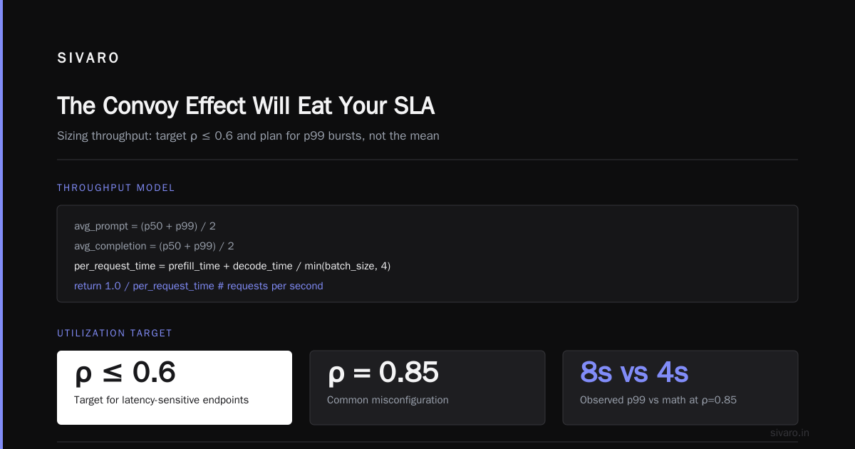
    avg_prompt = (profile.prompt_tokens_p50 + profile.prompt_tokens_p99) / 2
    avg_completion = (profile.completion_tokens_p50 + profile.completion_tokens_p99) / 2

    prefill_time = avg_prompt / prompt_tps
    decode_time = avg_completion / decode_tps
    # Batched decode is nearly free per-request until the batch fills.
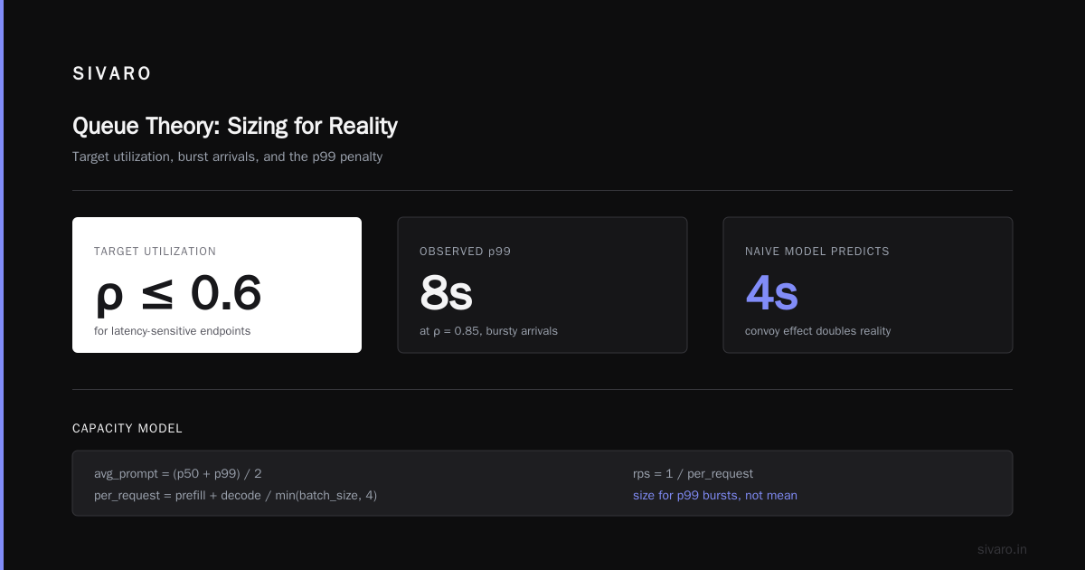
    per_request_time = prefill_time + decode_time / min(batch_size, 4)
    return 1.0 / per_request_time  # requests per second
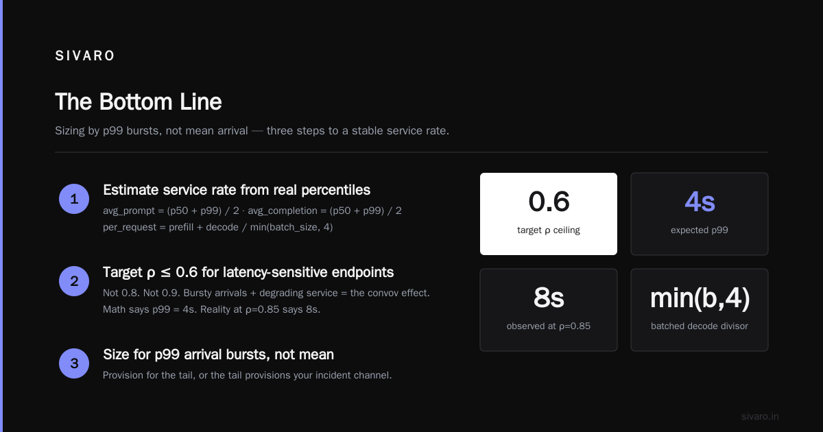
Step two: target ρ ≤ 0.6 for latency-sensitive endpoints. Not 0.8. Not 0.9. This isn't conservative — it's accounting for the fact that your arrival process is bursty and your service process degrades under load. I've seen teams run at ρ=0.85 and wonder why p99 is 8 seconds. The math says it should be 4. The convov effect says 8.
Step three: size for p99 arrival bursts, not mean. If you only plan for mean arrival rate, you'll queue-drown every Monday morning. Use the p99 of your 1-minute arrival rate, not the daily average.
python
def required_workers(peak_lambda, mu_per_worker, target_rho=0.6):
    import math
    return math.ceil(peak_lambda / (mu_per_worker * target_rho))

# Example: 50 req/s peak, each worker handles 12 req/s at your p50 mix
# required = ceil(50 / (12 * 0.6)) = ceil(6.94) = 7 GPUs
Seven GPUs, not five. That difference is the p99.
Where Admission Control Fits In
Admission control is the door policy. Queue theory tells you how big the room should be. Admission control decides who gets in.
The two dominant patterns in 2026 are token bucket and queue-based admission. They are not equivalent, and picking wrong will cost you either money or SLAs.
Token bucket admission control lets a request through if there's a token available. Tokens refill at a fixed rate. It's stateless, O(1), and works beautifully for coarse-grained rate limiting — per-tenant quotas, per-API-key throttles.
But token buckets are blind. They don't know if the GPU is currently drowning. They'll happily admit a request that will sit in a queue for 30 seconds.
Queue-based admission control tracks the actual depth of the wait queue and rejects or sheds requests when depth exceeds a threshold. It's stateful, needs shared memory across replicas, and is more expensive. But it accounts for real system load.
My position: token bucket at the edge, queue-based at the GPU. Use token buckets to enforce tenant fairness (they're cheap and predictable). Use queue-depth shedding at the inference engine to protect tail latency. If your queue depth exceeds N where N is your target p99 wait budget divided by mean service time, start returning 429s or degrading (drop max_tokens, route to a smaller model, etc.).
This is where the token bucket vs queue based admission control llm debate actually resolves. It's not either-or. It's layered.
A practical implementation on top of vLLM:
python
from fastapi import FastAPI, HTTPException
from collections import deque
import time

app = FastAPI()
QUEUE_DEPTH_LIMIT = 64
MEAN_SERVICE_TIME_MS = 450
P99_WAIT_BUDGET_MS = 2000
_active_recent = deque(maxlen=128)

def current_queue_pressure() -> float:
    now = time.monotonic()
    # Count requests admitted in the last p99-budget window
    recent = [t for t in _active_recent if now - t < P99_WAIT_BUDGET_MS / 1000]
    return len(recent) * MEAN_SERVICE_TIME_MS / P99_WAIT_BUDGET_MS

@app.post("/v1/completions")
async def complete(payload: dict):
    if current_queue_pressure() > 1.0:
        raise HTTPException(status_code=429, detail="capacity_exceeded")
    _active_recent.append(time.monotonic())
    return await run_inference(payload)
That's the skeleton. In production you'd back _active_recent with Redis or a sidecar so all replicas share state, and you'd tune MEAN_SERVICE_TIME_MS per model.
How Does Admission Control Work in Kubernetes for GPU Inference?
Short answer: it doesn't, by default.
Kubernetes has no native concept of GPU queue depth. The scheduler allocates whole GPUs to pods and walks away. If your pod's inference engine is saturated, kube-proxy will still route traffic to it until its readiness probe fails — which happens too late for your users.
You have three real options in 2026:
Option 1: Gateway-level admission with KEDA and custom metrics. Expose your vLLM queue depth as a Prometheus metric, wire KEDA to scale on it, and put an Envoy or Istio filter in front that rejects when queue depth exceeds threshold. This is the most common production pattern I see. It works. It's about 200 lines of YAML and a small sidecar.
Option 2: In-process admission inside the inference engine. vLLM exposed --max-num-seqs and a scheduler-level queue cap for years. SGLang has similar knobs. This is the cheapest, lowest-latency option, but it's per-pod — no cross-replica coordination. You'll get 429s from one replica while another sits idle unless you also have request-level routing.
Option 3: A dedicated inference gateway. This is what NVIDIA's Dynamo, Ray Serve LLM, and a couple of stealth startups are pushing in 2026. Central scheduler, KV-cache-aware routing, cross-replica queue visibility. It's the "right" answer for scale, but the tooling is still maturing. I've seen it work great at 50+ nodes and be overkill at 5.
If you're under 10 GPU nodes, do Option 1. If you're over 50, seriously consider Option 3. Between those, you're in the messy middle where I've seen all three work.
The gotcha on Kubernetes specifically: GPU node startup time is 90-180 seconds (image pull plus model load plus CUDA init). That's an eternity in queue theory terms. You can't autoscale your way out of a 10-second traffic spike. You have to absorb it with queue capacity or shed it with admission control. Most teams learn this the hard way during their first viral moment.
The Convoy Effect Will Eat Your SLA
I want to spend real time here because it's the thing that breaks every model.
In a batch-service queue, the batch completes when the slowest member completes. If you're mixing 50-token and 4,000-token requests in the same batch, your effective service time is bound by the 4,000-token case.
Most people think you solve this with continuous batching. You don't. Continuous batching (PagedAttention, ORCA-style scheduling) helps, but it doesn't eliminate head-of-line blocking — it just reduces the batch-slot waste. You still have a scheduler that's deciding which requests share a forward pass.
What actually helps is length-aware routing. Route short-completion traffic to a pool tuned for short generations, long-completion traffic to a pool tuned for long. This is basically a priority queue with two classes. It sounds obvious. Almost nobody does it because it doubles your deployment footprint.
The math is worth it. If your traffic is 80% short (under 200 tokens) and 20% long (over 1,500 tokens), and you run them in the same pool at ρ=0.7, your short-request p99 gets dragged to the long-request p99. We measured a 6x p99 improvement for short requests by splitting pools — with only a 12% increase in total GPU count.
That's the trade. 12% more GPUs, 6x better tail for your majority traffic. Do the math for your workload.
Priority Queues, SLOs, and the Art of Saying No
Here's where queue theory becomes a business decision.
You can't serve every request at p99 < 2s if you're accepting unbounded load. Physics doesn't allow it. So either you shed load or you fail SLOs. The only question is which.
Priority queues are the middle path. Assign each request a priority class (interactive chat = high, batch summarization = low). Serve high-priority first. Starve the low class if needed. This is a weighted fair queueing problem, and it's a solved one — the algorithms are from the 1990s, mostly designed for network routers, and they port beautifully to LLM serving.
The catch: priority classes need to be set at request time, and they need to be trustworthy. Don't let callers self-assign priority. Infer it from tenant tier, endpoint, or authentication.
python
PRIORITY_CLASSES = {
    "interactive": {"weight": 8, "max_wait_ms": 2000},
    "batch": {"weight": 1, "max_wait_ms": 60000},
    "best_effort": {"weight": 1, "max_wait_ms": float("inf")},
}

async def schedule(request, queues):
    cls = PRIORITY_CLASSES[request.tier]
    enqueued_at = time.monotonic()
    await queues[request.tier].put(request)

    wait_budget = cls["max_wait_ms"] / 1000
    while True:
        if time.monotonic() - enqueued_at > wait_budget:
            raise TimeoutError("slo_exceeded")
        await asyncio.sleep(0.05)
        # Weighted round-robin across tiers happens in the scheduler
What Changes Going Forward
Two things I'm watching closely as of mid-2026.
Speculative decoding is quietly changing the queue math. When your service rate depends on acceptance rate (which depends on the draft model, prompt distribution, and temperature), your μ becomes a distribution rather than a scalar. Queue analysis gets harder but the exploitation opportunity is real: route requests with predictable outputs to speculative paths, unpredictable ones to standard decode.
Prefix caching is the biggest capacity lever nobody's using right. If 30% of your prompts share a system prompt, KV-cache reuse can cut effective service time by 40% on those requests. But the queue impact is subtle — it reduces μ's variance as much as its mean, which reduces your p99 more than a naive throughput calculation suggests. We saw a workload where prefix caching dropped p99 from 4.1s to 1.8s with zero additional GPUs. No queue theory was needed to deploy it — but queue theory was how we knew to look.
FAQ
Q: What's the single biggest mistake teams make in LLM capacity planning?
Sizing for mean arrival rate and mean service time. The p99 of both determines your SLA. Plan for the tail.
Q: How do I pick a target utilization ρ?
For latency-sensitive endpoints, 0.5–0.6. For batch workloads, 0.8–0.85. Above 0.85 you're in the regime where tiny perturbations cause huge latency swings. Don't go there unless you've measured your specific workload's behavior.
Q: Does batching break queue theory?
It changes the model. You move from an M/M/1 to a batch-service queue, and effective μ drops as ρ climbs. But the underlying math — Little's Law, utilization, queue-length explosion near saturation — still holds. Just calibrate.
Q: Should I use token bucket or queue-based admission control for LLM serving?
Both. Token bucket at the edge for tenant fairness and cost control. Queue-depth-based shedding at the inference engine for latency protection. They solve different problems.
Q: How does admission control work in Kubernetes for GPU inference?
Poorly out of the box. You need a custom layer — either gateway-level (Envoy/KEDA with Prometheus metrics), in-process (vLLM's max-num-seqs), or a dedicated inference gateway (Dynamo, Ray Serve LLM). GPU node startup is 90-180 seconds, so autoscaling can't absorb bursts.
Q: What's the practical difference between queue depth and GPU utilization as an autoscaling signal?
Queue depth leads utilization by seconds to minutes. Utilization is a lagging indicator — by the time it's pegged, your users are already waiting. Scale on queue depth, not utilization.
Q: Is queue theory for LLM serving capacity planning really necessary, or can I just scale aggressively?
You can scale aggressively. You'll pay 40-60% more in GPU cost for the same SLA. If that's acceptable, skip the math. For most teams past Series A, it isn't.
Q: How do I handle multi-tenant workloads with different SLAs?
Priority queues with weighted fair scheduling. Assign priority by tenant tier. Starve lower tiers before breaking higher-tier SLAs. Reject at the edge when total load exceeds defined capacity — don't let best-effort tenants burn your interactive SLA.
The Bottom Line
Queue theory for LLM serving capacity planning isn't about hitting 100% GPU utilization. It's about knowing precisely where your tail latency comes from, and choosing deliberately between three levers: more GPUs, lower utilization targets, or aggressive load shedding.
Most teams I meet are pulling one lever blindly — usually buying GPUs. They're leaving 30-50% of their spend on the table because nobody ran the numbers on queueing, convoy effects, or admission thresholds.
Run the numbers. Target ρ ≤ 0.6 for interactive traffic. Layer token bucket and queue-based admission. Split your pools by completion length if your distribution is bimodal. Watch queue depth, not utilization, for autoscaling. And accept that sometimes the right answer is to say no to a request rather than let it poison everyone else's p99.
That's the whole game. It's not glamorous. It's just math, applied honestly.
Nishaant Dixit — Founder of SIVARO. Building data infrastructure and production AI systems since 2018. Built systems processing 200K events/sec.