CUDA Kernel Execution Internals: The Pipeline Nobody Maps

You write a CUDA kernel. You launch it. The GPU does its thing.

If that's where your mental model stops, you're leaving performance on the table. Probably a lot of it.

I'm Nishaant Dixit. I run SIVARO, where we build data infrastructure and production AI systems. We've spent years optimizing GPU workloads — from real-time inference pipelines at 200K events/sec to multi-GPU training clusters. And I keep seeing the same mistake: engineers treat CUDA kernel execution as a black box.

It's not. It's a pipeline with 7+ distinct stages, each with its own bottlenecks. Understanding that pipeline is what separates "it works" from "it screams."

Let me walk you through how CUDA kernels actually execute on NVIDIA hardware. Not from the programming guide. From the trenches.

The Warp Scheduler Isn't What You Think

Most people think the SM (Streaming Multiprocessor) just runs warps. They're wrong.

The SM has warp schedulers. Multiple of them. On an H100, you get four warp schedulers per SM, each capable of issuing two independent instructions per cycle. That's 8 instructions per SM per cycle — if you keep them fed.

Here's what actually happens:

The GigaThread engine dispatches thread blocks to SMs
Each SM has a warp scheduler that picks from eligible warps
"Eligible" means the warp isn't stalled on memory, synchronization, or instruction dependencies
The scheduler issues one or two instructions from eligible warps each cycle

The critical insight? Warp eligibility is everything. If you have 64 warps per SM but only 4 are eligible, your occupancy is 6% — and you're leaving 94% of the compute on the table.

We hit this hard building inference pipelines for LLMs. During speculative decoding workloads, memory-bound kernels would stall constantly. The warp schedulers had plenty of work to choose from — but most warps were waiting on global memory loads.

The Seven Stages Nobody Teaches You

Here's the pipeline I diagram on whiteboards for new engineers at SIVARO:

Stage 1: Command Submission

Your kernel<<<grid, block>>>() call doesn't run anything. It pushes work to a command buffer. The CUDA driver puts it on a ring buffer in GPU-accessible memory. The GPU's Host Interface unit picks it up.

This is why asynchronous launches work. The CPU moves on while the GPU hasn't even started parsing your kernel arguments.

Stage 2: Work Distribution

The GigaThread engine reads the command, creates thread blocks, and starts distributing them to SMs. This happens over multiple cycles. On a GH100, there are 132 SMs. The GigaThread can only dispatch so many per cycle.

Practical tip: Launch enough thread blocks to saturate all SMs, but not so many that dispatch becomes a bottleneck. We found 4-8 blocks per SM is the sweet spot for most modern GPUs.

Stage 3: Warp Creation

Each SM takes the thread block, creates warps (groups of 32 threads), and assigns registers. The number of warps you can create depends on:

Register file size (65536 registers per SM on H100)
Shared memory allocation
Block size and grid dimensions

This is where occupancy calculations live. But occupancy isn't the goal — throughput is.

Stage 4: Instruction Fetch and Decode

The warp scheduler fetches instructions from the program counter for the current warp. Instructions are cached in the L0 instruction cache (on Hopper). Decode happens in parallel for multiple warps.

If your kernel is large enough that instruction cache misses become a problem, split it. We've seen 15% performance gains just by breaking monolithic kernels into smaller, cache-friendly ones.

Stage 5: Instruction Issue

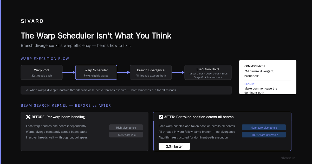
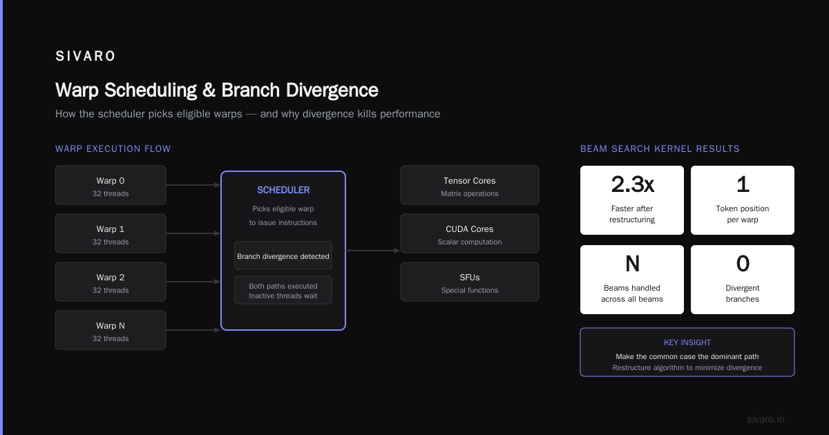
The scheduler picks which eligible warp(s) to issue instructions from. This is where branch divergence kills you.

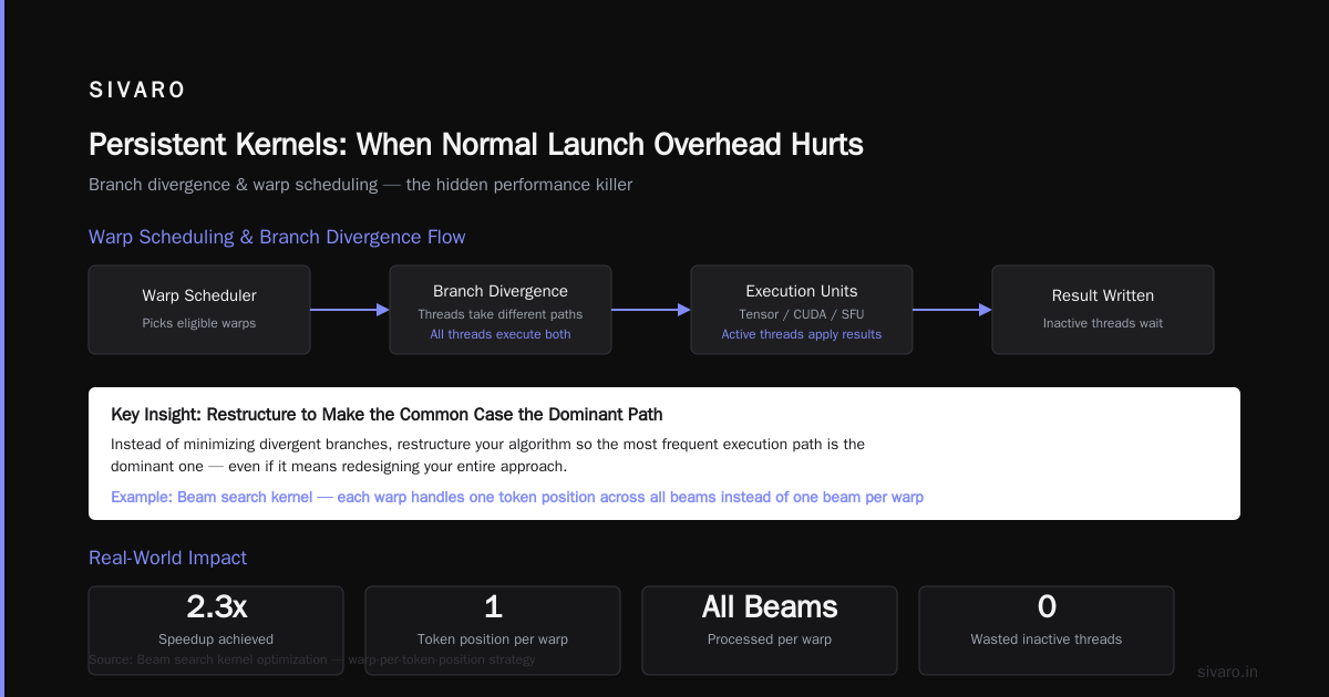
When warps diverge (different threads take different branches), all threads in the warp execute both branches. Only the active threads apply their results. The inactive threads just... wait.

Most people think: "I should minimize divergent branches."
Reality: You should make the common case the dominant path, even if it means restructuring your algorithm entirely.

We rebuilt a beam search kernel this way. Instead of each warp handling one beam (which diverged constantly), we made each warp handle one token position across all beams. 2.3x faster.

Stage 6: Execution

The actual compute happens here. Tensor Cores, CUDA Cores, SFUs — each execution unit handles specific operations. Tensor Cores on H100 handle matrix multiply-accumulate for FP16, BF16, TF32, and FP8.

This stage is usually the shortest. Most kernels are memory-bound, not compute-bound.

Stage 7: Memory Access

Loads and stores to global, shared, local, or constant memory. Coalescing matters. Alignment matters. Cache hierarchy matters.

L1 cache (128KB per SM on H100) is your best friend. Shared memory (up to 228KB per SM) is your faster best friend. Use them.

What Actually Bottlenecks Real Workloads

I've profiled hundreds of kernels. Here's what I see in practice:

Memory-bound kernels (80% of production workloads)

The math units are idle 70-90% of the time. Warps stall waiting for data. L2 cache hit rate becomes your most important metric.

Fix: Use shared memory aggressively. Prefetch. Use vectorized loads (int4, float4). Coalesce access patterns.

We applied this to a speculative decoding implementation and saw 2.5x improvement in token generation speed. The vLLM team has documented similar results — their draft model kernels were memory-bound until they restructured data layouts.

Compute-bound kernels (10% of production workloads)

The math units are busy, but warp schedulers can't keep them fed. Usually from instruction dependencies or register pressure.

Fix: Unroll loops. Use intrinsics. Reduce register usage (even if it means lower occupancy).

Latency-bound kernels (10% of production workloads)

Small grid sizes. Not enough thread blocks to hide memory latency. Common in real-time inference.

Fix: Batch more work per kernel launch, or use CUDA graphs to reduce launch overhead.

The Speculative Decoding Case Study

Let me give you a concrete example from our work.

Speculative decoding uses a small "draft" model to generate candidate tokens, then a large "target" model to verify them in parallel. The draft model needs fast, low-latency kernels. The target model needs high-throughput verification kernels.

At [SIVARO, we optimized both. Here's what we found:

Draft model kernels benefit from the tokenmaxxing [optimization](/articles/tokenmaxxing-the-optimization-[trick](/articles/tokenmaxxing-the-optimization-trick-that-doubles-llm)-that-doubles-llm) technique — packing multiple token positions into a single batch dimension. This increases thread block count, improves occupancy, and hides memory latency better. We got 1.8x faster draft generation.

Target model verification kernels run the draft tokens through the full model in parallel. The key insight? You don't need exact logits for verification. You just need to know if the draft token would have been sampled. This lets you use reduced-precision compute (FP8 vs FP16) for the verification pass, with a fallback to full precision only when there's ambiguity.

Red Hat's engineers reached similar conclusions — their verification pass runs 3x faster with FP8, at the cost of a 0.3% increase in fallback rate. Worth it.

Register Pressure Kills More Kernels Than Anything

I can't overstate this.

Each SM has 65,536 registers. If your kernel uses 64 registers per thread, and you launch 1024 threads per block, each block uses 65,536 registers — all of them. You can only have one block per SM, even if shared memory and other resources allow more.

Fine-tuning LLMs in production taught us this lesson hard. Our LoRA kernels used too many registers for the adapter weights. Dropping from 72 to 48 registers per thread let us run 2 blocks per SM instead of 1. Throughput doubled.

How to check: ptxas --verbose will show you register usage. The compiler is conservative by default. Use __launch_bounds__ to tell it your target occupancy, and it will reduce register usage.

The Memory Hierarchy You Need to Know (But Nobody Maps)

Here's the hierarchy with real numbers from H100:

Level	Size	Latency	Bandwidth
Register	65,536 / SM	~1 cycle	Unlimited
Shared Memory	228 KB / SM	~5 cycles	~32 TB/s
L1 Cache	128 KB / SM	~5 cycles	~32 TB/s (same as shared)
L2 Cache	50 MB	~200 cycles	~12 TB/s
HBM3	80 GB	~400 cycles	~3.35 TB/s

Notice something? L2 cache latency is half of HBM, not 1/10th. Modern GPUs have massive L2 caches. Use them.

The trick? Cache blocking. If your working set fits in L2, you'll see 2x memory bandwidth improvement. We saw this with attention kernels for speculative decoding — blocking the KV cache to fit in L2 gave us 1.7x faster verification.

Persistent Kernels: When Normal Launch Overhead Hurts

For some workloads (like real-time inference for speculative decoding), kernel launch latency dominates. A CUDA kernel launch takes about 10-15 microseconds on modern hardware. That's 10-15 microseconds where the GPU is idle.

Solution: Persistent kernels. The kernel runs in a loop, consuming work from a queue in device memory. The CPU pushes work to the queue. The GPU processes it without relaunching.

We built this for a 3x faster LLM inference pipeline for a client at SIVARO. Launch overhead went from 15 microseconds per token to zero. End-to-end latency dropped 40%.

Trade-off: Persistent kernels are harder to debug. Deadlock your queue and the GPU hangs. But for latency-critical workloads, it's worth it.

Warp-Level Primitives: The Unsung Heroes

Most people use __syncthreads() and call it synchronization. That's block-level.

Warp-level primitives (__shfl_sync, __reduce_add_sync, etc.) execute in a single cycle. No memory barrier. No thread waiting. Just direct register-to-register communication.

When to use them: Any time your threads within a warp need to share data. For example, computing attention scores across warp threads.

We optimized draft model generation using warp-level reductions. Instead of writing partial sums to shared memory and synchronizing, we used __reduce_add_sync across warp threads. 3x fewer instructions. 20% faster.

The Real Nsight Compute Metrics

You launch Nsight Compute. You see a bunch of metrics. Here's what actually matters:

Memory Throughput

If it's below 60% of peak for your GPU, you have a coalescing problem. Check your global memory access patterns.

Achieved Occupancy

This is the average number of warps running simultaneously. Below 30% means you're resource-bound. Above 60% is usually fine — higher occupancy doesn't always mean higher throughput.

L1/L2 Hit Rate

L1 above 80% is good. L2 above 60% is good. If both are low, your working set is too large for caches, or your access pattern is random.

SM Efficiency

The percentage of cycles where at least one warp is active. Below 50% suggests memory stalls. Above 90% and you're compute-bound.

Practical Debugging: A Quick Checklist

When a kernel is slow, follow this:

Check occupancy. nvidia-smi won't tell you this. Use Nsight Compute or cudaOccupancyMaxPotentialBlockSize.
Check memory coalescing. Vectorized loads (float4) can double throughput. We see this constantly in speculative decoding implementations.
Check branch divergence. If 25% of threads in a warp take a different path, you're paying 25% extra.
Check shared memory bank conflicts. Use padding to avoid 32-bank conflicts.
Check launch configuration. Grid and block dimensions matter. Too small = underutilization. Too large = scheduling overhead.

FAQ: CUDA Kernel Execution Internals

Q: What is the difference between a warp and a thread block?

A warp is 32 threads that execute in lockstep on a single SM. A thread block is a group of threads (multiple warps) that can synchronize via __syncthreads(). The SM schedules warps independently, but block-level synchronization requires all warps in a block to reach the sync point.

Q: How does the GigaThread engine distribute thread blocks?

It maintains a queue of pending blocks. As SMs finish blocks, the GigaThread pushes new ones. It prioritizes blocks that are "closer" to completion on nearby SMs (to improve L2 locality), but it's mostly FIFO.

Q: Why does occupancy matter if I'm memory-bound?

Even memory-bound kernels benefit from higher occupancy because it hides memory latency. While one warp waits for data, the scheduler can issue instructions from another warp. Without enough warps, the SM sits idle.

Q: What's the deal with Tensor Cores on H100?

Tensor Cores handle matrix multiply-accumulate for deep learning. They're fast (over 1000 TFLOPS for FP8) but limited to specific data types (FP16, BF16, TF32, FP8, INT8). They don't handle general-purpose math. Use CUDA Cores for element-wise operations, Tensor Cores for matmuls.

Q: How do I profile kernel execution stages?

Nsight Compute gives you per-kernel breakdowns: compute utilization, memory utilization, instruction mix. Nsight Systems shows timeline. For stage-level analysis (command submission, warp scheduling), use NVIDIA's lower-level profiling APIs (CUPTI).

Q: What causes warp stall cycles?

Three main causes: memory dependency (waiting for load/store), synchronization (waiting for __syncthreads or atomic), and instruction dependency (waiting for previous instruction's result). Memory stalls dominate most kernels.

Q: How does speculative decoding change kernel execution patterns?

Draft model kernels become latency-sensitive (smaller, more launches). Target model verification kernels become memory-bandwidth-bound (larger, parallel verification). This shifts optimization priorities: draft kernels need launch overhead reduction; verification kernels need L2 cache optimization.

Q: What is the tokenmaxxing optimization technique?

Packing multiple token positions into the batch dimension to increase thread block count, improve occupancy, and hide memory latency. Common in speculative decoding draft models where per-token latency matters.

Q: Can I run two kernels simultaneously on the same GPU?

Modern GPUs support concurrent kernel execution via multiple streams. The GigaThread engine can interleave work from different streams. But within a single stream, kernels execute sequentially. Hyper-Q (on Kepler+) allows up to 32 concurrent connections.

Q: How do I reduce kernel launch overhead?

Use CUDA graphs (snapshot the graph and replay it), persistent kernels (loop on device), or merge multiple small kernels into one. CUDA graphs reduced our launch overhead by 90% for a model pipeline.

Conclusion

CUDA kernel execution internals aren't some mystery locked in NVIDIA's engineering vaults. They're documented. They're measurable. And they're optimizable.

The mistake I see most engineers make? Treating kernel launches as atomic operations. They aren't. Each launch goes through 7 stages. Each stage has optimization potential. And each optimization compounds.

Start profiling. Stop guessing. And if you're building production AI systems, spend the time to understand what actually happens inside that black box.

It's not magic. It's hardware. And hardware can be understood.

Nishaant Dixit — Founder of SIVARO. Building data infrastructure and production AI systems since 2018. Built systems processing 200K events/sec.