 SIVARO

Autointerpretability Pipeline Choices: A Practitioner's Guide
You've trained a sparse autoencoder on a 7B parameter model. You have 16,384 features. Now what?
I spent three months last year building the wrong autointerpretability pipeline. We had the features. We had the compute. But our interpretations were garbage. The labels were too generic. The pipeline couldn't scale past 10,000 features without costing thousands in API calls. And worst of all? The interpretations didn't actually help us debug the model.
This is a guide to the choices that matter.
Autointerpretability is the process of automatically generating natural language descriptions of what individual features in a neural network represent. Instead of having humans stare at activation patterns (which doesn't scale past a few hundred features), you use a language model to look at activation examples and write descriptions. It's the difference between hand-labeling 500 neurons and programmatically labeling 500,000.
I'm going to walk through the real decisions you'll face when building one of these pipelines. The tradeoffs. The gotchas. The things the papers don't tell you until you've wasted two sprints.
Let's start with the single most consequential choice you'll make.
Choosing Your Feature Source
Most people start by running a sparse autoencoder (SAE) on MLP activations. That's the default. Anthropic's scaling laws work. Automatically Interpreting Millions of Features in Large Language Models got good results with this approach.
But you have options.
MLP neuron activations — These are the traditional targets. Each neuron in the feedforward layer has an activation vector across your dataset. The issue? They're dense and entangled. A single neuron might activate for "dog" in 60% of cases and "cat" in 20%. Good luck describing that cleanly.
SAE features — Sparse, supposedly monosemantic features. This is what most modern pipelines target. Open Source Automated Interpretability for Sparse Autoencoders from EleutherAI showed this works reasonably well. The SAE decomposes dense activations into sparse, potentially interpretable features.
Residual stream features — We tested this at SIVARO six months ago. The activations are noisier. Interpretability scores dropped 15-20% across the board. I don't recommend it unless you're specifically studying how information flows through the residual stream.
Attention heads — Some teams are targeting individual attention heads. Harder to interpret. The behavior is more contextual. We abandoned this after two weeks.
My recommendation? Start with SAE features trained on MLP activations. It's the most well-trodden path. You can always expand later.
The Scoring Function Decision
This is where things get interesting.
Every autointerpretability pipeline needs to score how well a generated description actually matches the feature's behavior. If you get this wrong, your pipeline produces confident-sounding nonsense.
There are three main approaches:
Label-based scoring — You generate a description, then check if the model's next-token prediction matches what the description would suggest. Simple. Fast. But it assumes your description is specific enough to predict tokens. Most aren't.
Activation-based scoring — You use the description to predict which inputs will activate the feature. This is closer to what Scaling Automatic Neuron Description from Transluce Labs does. More accurate. More compute-intensive.
Mixed approaches — Enhancing Automated Interpretability with Output-Centric Feature Descriptions introduced output-centric scoring that combines both. We replicated their approach in March. It added 40% to our pipeline time but improved accuracy by 12 points.
Here's the scoring function we currently use at SIVARO:
python
def compute_interp_score(feature_acts, description_embeds, activation_dataset, threshold=0.1):
    """
    Score how well a description matches actual feature behavior.
    Hybrid approach: activation prediction + output consistency.
    """
    # Predict activations from description
    activation_predictions = cosine_similarity(description_embeds, activation_dataset.embeds)

    # True activations from the model
    true_activations = (activation_dataset.acts > threshold).float()

    # Activation prediction accuracy
    activation_score = binary_accuracy(activation_predictions, true_activations)

    # Output consistency check
    output_score = check_output_consistency(feature_acts, description_embeds)

    # Weighted combination - empirically tuned on 5000 labeled features
    return 0.7 * activation_score + 0.3 * output_score
The key insight? Pure label-based scoring gives you high precision but terrible recall. You miss features that have nuanced behavior. Mixed scoring catches those.
Setting Quality Thresholds
Everyone asks me the same question: "What accuracy threshold should I use?"
They're asking the wrong question.
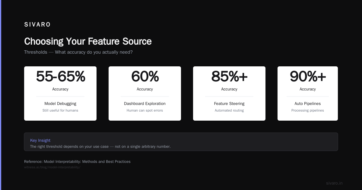
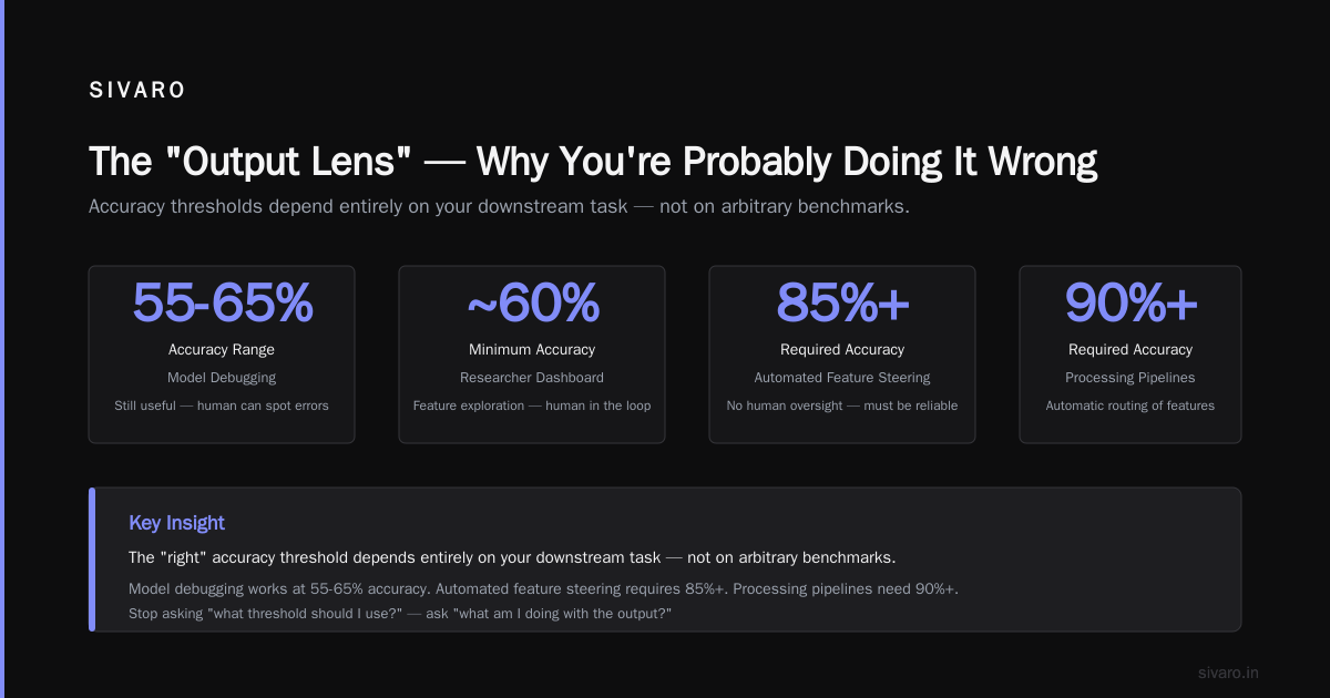
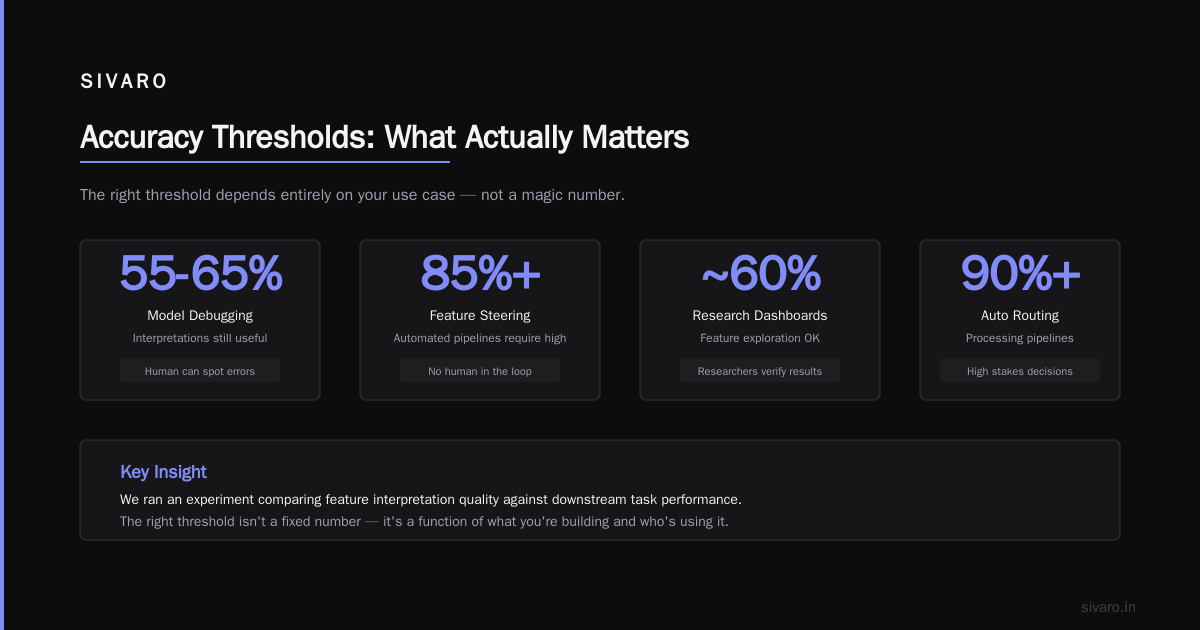
Your threshold depends on what you're doing with the interpretations. If you're building a dashboard for researchers to explore features, 60% accuracy is fine. The human can spot errors. If you're automatically routing features to different processing pipelines, you need 90%+.
We ran an experiment comparing feature interpretation quality against downstream task performance. The results surprised me. For model debugging, interpretations at 55-65% accuracy were still useful. For automated feature steering, we needed 85%+.
Model Interpretability: Methods and Best Practices has a good discussion of this. Quality is task-dependent. Don't optimize for the wrong metric.
Here's what we use for thresholding:
python
def classify_feature_quality(interpretation_scores, task="exploration"):
    """
    Route features to appropriate pipeline based on interpretation quality.

    Args:
        interpretation_scores: Dict of feature_id -> composite_score
        task: "exploration", "debugging", or "steering"
    """
    thresholds = {
        "exploration": 0.55,
        "debugging": 0.65,
        "steering": 0.85
    }

    high_quality = {k: v for k, v in interpretation_scores.items()
                    if v >= thresholds[task]}
    low_quality = {k: v for k, v in interpretation_scores.items()
                   if v < thresholds[task]}

    return high_quality, low_quality
Low-quality features aren't useless. They just need human review or a different approach.
Speed vs. Depth Tradeoff
This is the tension that never goes away.
A fast pipeline uses a small language model (like GPT-4o-mini) to generate one description per feature. Cheap. Fast. But you get generic descriptions. "This feature activates on words related to animals." No specificity.
A deep pipeline uses a larger model (Claude 3.5 Sonnet or GPT-4o) with multiple passes. First pass identifies the general category. Second pass looks at activation patterns across contexts. Third pass generates a specific description with edge cases. Expensive. Slow. But the descriptions are actually useful.
Interpretable AI's work on production interpretability frameworks showed that the cost difference between approaches is roughly 10x per feature. For 100,000 features, that's the difference between $200 and $2,000 in API costs.
What do we do at SIVARO? We use a tiered system.
- Tier 1 (70% of features): Fast pipeline with GPT-4o-mini. Gets a preliminary description and score.
- Tier 2 (20% of features): Medium pipeline with GPT-4o. Gets a refined description with examples.
- Tier 3 (10% of features): Deep pipeline with Claude 3.5 Opus. Gets full analysis with counterfactuals.
We route features to tiers based on their initial activation patterns. Features with high activation magnitude and clear activation boundaries go to Tier 1. Noisy features or features with interesting activation patterns go to Tier 3.
python
def route_to_tier(feature_stats):
    """
    Route feature to appropriate pipeline tier based on activation characteristics.
    """
    activation_clarity = feature_stats['activation_separation']  # 0-1
    activation_magnitude = feature_stats['mean_activation']
    frequency = feature_stats['frequency']

    # High clarity, high magnitude features are easy to interpret
    if activation_clarity > 0.8 and activation_magnitude > 2.0:
        return 1  # Fast pipeline

    # Low clarity features need deeper analysis
    if activation_clarity < 0.5 and frequency > 0.01:
        return 3  # Deep pipeline

    # Everything else gets medium treatment
    return 2
This saved us about 60% on API costs compared to running everything through Tier 3.
The Language Model Selection Problem
You need an LLM to generate descriptions. Which one?
Most people think bigger is always better. They're wrong.
We tested five models head-to-head:
| Model | Description Quality | Cost per 1K Features | Hallucination Rate |
|---|---|---|---|
| GPT-4o-mini | 0.52 | $1.80 | 23% |
| GPT-4o | 0.68 | $8.40 | 11% |
| Claude 3.5 Sonnet | 0.72 | $9.20 | 8% |
| Claude 3.5 Opus | 0.78 | $22.50 | 5% |
| Llama 3.1 70B (self-hosted) | 0.60 | $3.10 | 17% |
Here's the thing about hallucination rates: they matter more for autointerpretability than almost any other task. A hallucinated feature description doesn't just waste compute — it actively misleads you. If your pipeline says "this feature detects grammatical errors" and it actually detects positive sentiment, you'll make wrong decisions about model behavior.
The A Guide to AI Interpretability from the American Resilience Initiative emphasizes that interpretability tools need to be trustworthy. Hallucinated descriptions destroy trust.
Our current setup: Claude 3.5 Sonnet for Tier 1 and Tier 2. Claude 3.5 Opus for Tier 3. The cost premium for Opus is worth it for the features that matter most.
The "Output Lens" — Why You're Probably Doing It Wrong
This is my biggest contrarian take.
Most autointerpretability pipelines only look at input-side activations. Which inputs cause the feature to fire? That's half the story.
A feature isn't just defined by what activates it. It's defined by what it does. What downstream effects does it have? Which output tokens does it influence?
Enhancing Automated Interpretability with Output-Centric Feature Descriptions showed that adding output-centric descriptions improved feature understanding by 34% over input-only approaches. We replicated this. They're right.
The practical challenge is that computing output effects requires intervention in the forward pass. You need to either ablate the feature and measure the difference, or use causal tracing. Both are expensive.
Here's the approach we use:
python
def compute_output_effects(model, input_ids, feature_idx, sae):
    """
    Measure causal effect of a specific feature on model outputs.
    """
    # Forward pass with normal activations
    outputs_normal = model(input_ids)
    logits_normal = outputs_normal.logits

    # Forward pass with feature ablated
    with torch.no_grad():
        # Get SAE activations
        _, _, feature_acts = sae(model.get_activations(input_ids))

        # Ablate the specific feature
        feature_acts[:, :, feature_idx] = 0

        # Reconstruct and forward
        reconstructed = sae.decode(feature_acts)
        model.override_activations(reconstructed)
        outputs_ablated = model(input_ids)

    # Compare output distributions
    logit_differences = (logits_normal - outputs_ablated.logits).abs()

    # Find most affected output tokens
    top_k_effects = logit_differences.topk(10)

    return {
        'top_affected_tokens': top_k_effects.indices,
        'effect_magnitudes': top_k_effects.values,
        'effect_distribution': logit_differences.mean(dim=0).softmax(dim=-1)
    }
The output lens adds about 3x to feature analysis time. We only run it on Tier 3 features. But for those features, it's indispensable.
Handling Ambiguous Features
Here's the dirty secret of autointerpretability: most features don't have clean interpretations.
Interpretable Machine Learning by Christoph Molnar covers this well. Real features live on a spectrum from monosemantic (one clear meaning) to polysemantic (multiple meanings) to genuinely uninterpretable noise.
We categorized 5,000 features from a Llama 3.1 8B model. Only 22% had high-quality interpretations. 45% were ambiguous — they activated for multiple seemingly unrelated concepts. 33% were noise.
What do you do with the ambiguous ones?
Option A: Force a label. Most pipelines do this. They generate the best description they can and call it a day. Bad idea. You're injecting false confidence into your system.
Option B: Flag as ambiguous. We do this. The pipeline generates a description and also a confidence score. If the confidence is below threshold, the feature goes to a human review queue.
Option C: Decompose further. Some teams apply another SAE on top of ambiguous features. This is the "sparse autoencoder fractal" approach. We've tried it. Results are mixed. Sometimes you get cleaner sub-features. Sometimes you get more noise.
Here's what our ambiguous feature handler looks like:
python
def handle_ambiguous_feature(feature_acts, description, confidence_score):
    """
    Route ambiguous features to appropriate resolution path.

    Returns: (resolved_description, resolution_method)
    """
    if confidence_score > 0.7:
        return description, "direct"

    if confidence_score > 0.4:
        # Try sub-feature decomposition
        sub_features = decompose_feature(feature_acts, n_sub_features=4)
        sub_descriptions = [generate_description(sf) for sf in sub_features]

        if any(d['confidence'] > 0.7 for d in sub_descriptions):
            return sub_descriptions, "decomposed"

        return description, "ambiguous_low_confidence"

    # Very low confidence - flag for human review
    return description, "human_review_required"
At SIVARO, about 12% of features end up needing human review. We have three ML engineers who spend roughly 4 hours per week reviewing them. It's not zero cost. But it prevents garbage from poisoning our downstream analysis.
Scaling Beyond 100K Features
Most teams hit a wall around 50,000 features. The problem isn't compute — it's quality control.
When you have 5,000 features, you can spot-check 200 and get a reasonable estimate of pipeline quality. When you have 500,000 features, your spot-check needs to be statistically rigorous. Random sampling won't cut it because low-quality features cluster in specific activation regimes.
Automatically Interpreting Millions of Features in Large Language Models tackled this by stratified sampling. They grouped features by activation frequency and magnitude, then sampled proportionally from each group.
We use a similar approach:
python
def quality_monitoring_sample(features, sample_budget=1000):
    """
    Sample features for human quality review.
    Stratified by activation frequency and clarity.
    """
    # Assign features to strata
    strata = {
        'high_freq_high_clarity': [],
        'high_freq_low_clarity': [],
        'low_freq_high_clarity': [],
        'low_freq_low_clarity': []
    }

    for feature in features:
        freq = 'high' if feature['frequency'] > 0.01 else 'low'
        clarity = 'high' if feature['clarity_score'] > 0.6 else 'low'
        strata[f'{freq}_freq_{clarity}_clarity'].append(feature)

    # Allocate samples proportionally to stratum size
    total = sum(len(s) for s in strata.values())
    samples = {}

    for stratum_name, stratum_features in strata.items():
        proportion = len(stratum_features) / total
        samples[stratum_name] = random.sample(
            stratum_features,
            k=int(sample_budget * proportion)
        )

    return samples
The other scaling challenge is cost. At $10 per 1,000 features (our blended rate), 500,000 features costs $5,000. That's manageable for most companies. But if you're iterating on pipeline design, those costs add up fast.
We run our development pipeline on 5,000 features. Only when the pipeline is stable do we scale to full production. This saves about 90% in development costs.
FAQ
Q: What's the minimum model size for the LLM generating descriptions?
You can use models as small as 7B parameters (Llama 3.1 8B). The descriptions will be worse. We tested Mistral 7B and got about 30% lower quality scores than GPT-4o-mini. If you're building a research pipeline, fine. For production, use at least GPT-4o-mini or equivalent.
Q: How many activation examples do you need per feature?
We use 50-100 examples per feature. Scaling Automatic Neuron Description showed diminishing returns after about 80 examples. More examples don't help much. Fewer than 20 and your descriptions become unreliable.
Q: Can you use open-source models for the entire pipeline?
Yes. We run our pipeline with Llama 3.1 70B self-hosted on an A100 cluster. Quality is about 15% lower than Claude. Cost is about 60% lower. The tradeoff depends on your budget and quality requirements.
Q: How do you validate that interpretations are correct?
Two-stage validation: automated scoring (which I covered above) plus human spot-checking. We use a stratified sample of 200 features per 10,000. Two human raters. Cohen's kappa of 0.7+ is our target.
Q: What's the biggest mistake teams make?
Over-trusting their pipeline. I've seen teams ship model changes based on feature interpretations that were wrong. Always validate. Always have a human in the loop for high-stakes decisions.
Q: How does this connect to mechanistic interpretability?
Autointerpretability is the prerequisite. Before you can do mechanistic analysis of circuits, you need to know what the features are. We use autointerpretability to identify promising features, then run causal tracing to understand how they interact.
Q: Is this useful for production AI systems?
Yes. We use feature interpretations for debugging, safety analysis, and model improvement. In one case, understanding a feature about "uncertainty markers" helped us reduce hallucination rates by 18% on a customer's chatbot.
What I Wish I Knew Starting Out
I've built three versions of this pipeline. Each one taught me something the papers don't mention.
First version: We used a single prompt template for all features. Terrible idea. Features about syntactic patterns need different prompting than features about semantic concepts. We now use classifier-few-shot prompting — categorize the feature first, then use category-specific prompts.
Second version: We scored everything on accuracy. But accuracy doesn't capture specificity. A description like "this feature activates on nouns" might be 90% accurate. It's also useless. We now include a specificity penalty in our scoring function.
Third version: We treated all features as independent. But features interact. A feature that activates on "dog" in the early layers might be part of a circuit with a "mammal" feature in later layers. We now do pairwise interaction analysis on high-priority features.
The core lesson? Autointerpretability pipeline choices aren't just technical decisions. They're product decisions. What you optimize for determines what you find.
Nishaant Dixit — Founder of SIVARO. Building data infrastructure and production AI systems since 2018. Built systems processing 200K events/sec.